Optimal Execution With Limit Price

A simple Hamilton-Jacobi-Bellman approach

Say we want to buy Q=10,000 shares of a stock (initial price s_0=$20) with a maximum price $20.25. We want to find the cheapest possible way to do this. Clearly, the closer the stock price gets to the limit, the faster we want to buy. So, if our speed of trading is modeled as a function of the stock price and our current position (it could conceivably depend on other variables, but that’s the minimal dependency), that function must be increasing in the stock price, and must become infinite when the price approaches the limit, if we haven’t bought all the shares we need.

The question is: what is the best function we should use? This is a classic problem, which has been solved in a number of different ways, along with numerous possible extensions. What I want to present here is, in my opinion, the simplest possible way to arrive at a closed-form solution, under basic assumptions: Brownian stock price, linear temporary market impact, no permanent impact.

In this framework, the stock’s mid price s, the negative inventory q = Q minus our current inventory (so that we start at q0 = Q and end up at 0), and the cash account x, are processes that satisfy:

\(\begin{equation*} (1) \left\{ \begin{split} ds_t &= \sigma dW_t\\ dq_t &= -\lambda_t dt\ \ \ q_0=Q,\ dq_t\le 0,\ \lambda_t\ge 0,\\ d x_t &= -(s_t + \delta + \theta \lambda_t)\lambda_t dt,\\ \end{split} \right. \end{equation*} \)

where δ>0 is a constant half-spread we pay above mid, θ>0 represents the linear market impact, and λ_t >= 0 is the speed of buying (shares per unit of time). Since we want to buy a fixed number of shares Q, a fixed cost Qδ is incurred whatever the trading strategy. To determine the optimal strategy, we can therefore, without loss of generality, set δ = 0, and maximize our expected pnl (that is, minimize our cost):

\(\begin{split} &u(s,x,q,t) = \sup_{\{\lambda_t\},\ q_\tau = 0}\mathbb{E}\left(x_\tau - q_\tau s_\tau\right),\\ \\ &\hbox{where }\tau \hbox{ is the stopping time }s_\tau=\overline{s}\hbox{ (maximum price)}\\ \end{split} \)

Note the minus sign for q_τ s_τ in the pnl, since q here is Q minus our stock inventory (for convenience).

It is standard that u satisfies the Hamilton-Jacobi-Bellman equation associated to the SDE’s (1):

\(\begin{equation*} (2) \left\{ \begin{split} &u_t + \frac{\sigma^2}{2}u_{ss} + \sup_\lambda\left(-\lambda u_q - (s+\theta\lambda)\lambda u_x\right) = 0\\ \\ &u(\overline{s},x,q,t)= -\infty\ \ \hbox{ if } q>0\\ \\ &u(\overline{s},x,0,t) = x\\ \end{split} \right. \end{equation*} \)

Note how the constraint that q be zero when s reaches the limit price is enforced via penalization in the infinite boundary condition. We won’t worry too much about technical details; our goal here is to compute an explicit solution to (2). For that, we make the following ansatz:

\((3) \ \ \ u(s,x,q,t) = x - sq +h(s) q^2\)

which, since u_x = 1 and u_t = 0, leads to

\(\begin{equation*} (4) \left\{ \begin{split} &\frac{\sigma^2}{2}u_{ss}-\inf_{\lambda}\left(\theta\lambda^2 + (s+u_q)\lambda\right) = 0\\ &\hbox{optimal strat}\ \ \lambda^* = -\frac{1}{2\theta}(s + u_q)\\ \end{split} \right. \end{equation*} \)

and, computing u_q from (3):

\(\begin{equation*} \left\{ \begin{split} &\frac{\sigma^2}{2}h’’(s) + \frac{1}{\theta}h^2(s) = 0\\ \\ &h(\overline{s}) = -\infty \end{split} \right. \end{equation*} \)

This leads to

\(\begin{split} &\frac{\sigma^2\theta}{4}h’^2 + \frac{1}{3} h^3 = \hbox{Const}\\ \\ &\hbox{and since }h(-\infty) = h’(-\infty) = 0,\ \hbox{we have }\ \hbox{Const} = 0,\\ \end{split} \)

which, in turn, allows us to solve for h, and, from there, for the optimal trading strategy — optimal speed of trading λ* —

\(\begin{equation*} (5) \left\{ \begin{split} &h(s) = -\frac{3\sigma^2\theta}{\left(\overline{s} - s\right)^2}\\ \\ &\lambda^* = \frac{3\sigma^2q}{\left(\overline{s} - s\right)^2} \end{split} \right. \end{equation*} \)

As expected, if we still have shares to buy q>0 when the stock price s is close to reaching our maximum price, our speed of trading λ* increases in order to meet our goal. What is perhaps less intuitive is that the speed should increase as the negative power of two of the distance to the max price — although you could arrive at that result by a straightforward dimensional analysis. Aside from that, our speed of trading is proportional to the remaining number of shares to be bought, as well as to the stock variance.

Let’s see in practice how this optimal solution beats other strategies. For this, we run a Monte-Carlo simulation with different speed of trading functions, and compute the average cost (which is just negative the pnl, defined above) (time unit = 1 minute, horizon = 1 day):

We now compare the performance of the optimal speed of trading λ* to speed functions with a power of the distance to the limit price that is different from -2, namely: -1/2, -1, -3. Here are the results:

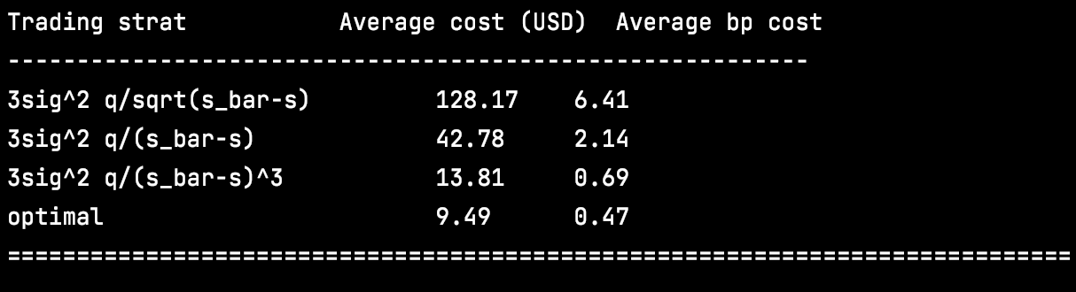
This is the cost of trading above and beyond a constant half-spread; in other words, the cost of market impact. As expected from the theoretical result in (5), the best speed of trading function is the power -2 (“optimal” in the printout above).

The python code used to generate the results above is available below the fold to paying subscribers.

Quantitatively Yours,

---

from __future__ import print_function
import numpy as np
import matplotlib.pyplot as plt

DisplayPlots = False
NIter = 100000
s0 = 20.
s_bar = 20.25
Q = 10000
T = 1.
nt = 1440
delta_t = T/nt
sigma = s0 * 0.02
theta = 0.5e-5  * delta_t
Scenarios = ['3sig^2 q/sqrt(s_bar-s)','3sig^2 q/(s_bar-s)','3sig^2 q/(s_bar-s)^3','optimal']
ns = len(Scenarios)
ExpPnl = np.zeros(ns)
if DisplayPlots:
    n_traj = 10
    Display_s = np.zeros((nt,n_traj))
    Display_q = np.zeros((nt,n_traj))
    Display_pnl = np.zeros((nt,n_traj))
for s_ind in range(ns):
    ExpPnl[s_ind] = 0
    np.random.seed(100)
    for n in range(NIter):
        if n % 1000 == 0:
            print("s_ind=%d, n=%d"%(s_ind,n))
        s = np.zeros(nt)
        q = np.zeros(nt)
        x = np.zeros(nt)
        pnl = np.zeros(nt)
        eps = np.random.normal(0, 1, nt)
        s[0] = s0
        q[0] = Q
        for t in range(1,nt):
            epsilon = 1e-10
            if s_ind == 0:
                lam = 3 * sigma ** 2 * q[t-1] / np.sqrt(max(s_bar - s[t-1],epsilon))
            if s_ind == 1:
                lam = 3 * sigma ** 2 * q[t-1] / max(s_bar - s[t-1],epsilon)
            if s_ind == 2:
                lam = 3 * sigma ** 2 * q[t-1] / max(s_bar - s[t-1],epsilon)**3
            if s_ind == 3:
                lam = 3 * sigma ** 2 * q[t-1] / max(s_bar - s[t-1],epsilon) ** 2
            q[t] = max(q[t-1] - round(delta_t * lam),0)
            dq = q[t] - q[t-1]
            x[t] = x[t-1] + (s[t-1] - theta * (dq / delta_t) ) * dq
            s[t] = s[t-1] + sigma * eps[t] / np.sqrt(nt)
            pnl[t] = x[t] + (Q - q[t]) * s[t]
            #print("s=%1.2f, lam=%1.2f, q=%d, x=%1.2f, pnl=%1.2f"%(s[t-1],lam,q[t],x[t],x[t] + (Q-q[t])*s[t-1]))
        if DisplayPlots and ( s_ind == 3) and ( n < n_traj ):
            Display_s[:,n] = s
            Display_q[:, n] = q
            Display_pnl[:,n] = pnl
        ExpPnl[s_ind] += x[-1] + (Q-q[-1]) * s[-1]
    ExpPnl[s_ind] /= NIter
print("Trading strat\t\t\tAverage cost (USD)\tAverage bp cost")
print("----------------------------------------------------------")
for s_ind in range(ns):
    print('{:30s} {:1.2f} \t {:1.2f}'.format(Scenarios[s_ind],-ExpPnl[s_ind],-1e4 * ExpPnl[s_ind] / (s0 * Q)))
print("=============================================================================")

if DisplayPlots:
    plt.figure()
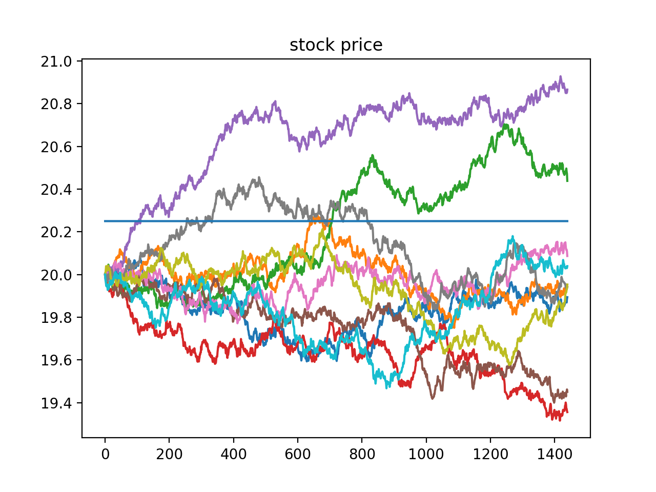
    plt.plot(Display_s)
    plt.plot(s_bar * np.ones(nt))
    plt.title('stock price')
    plt.figure()
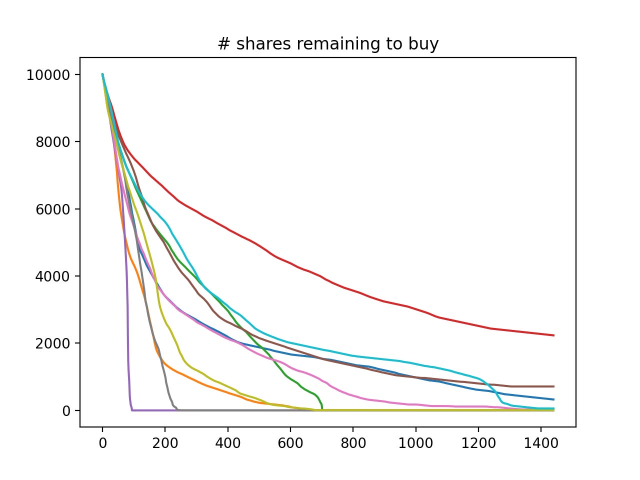
    plt.plot(Display_q)
    plt.title('# shares remaining to buy')
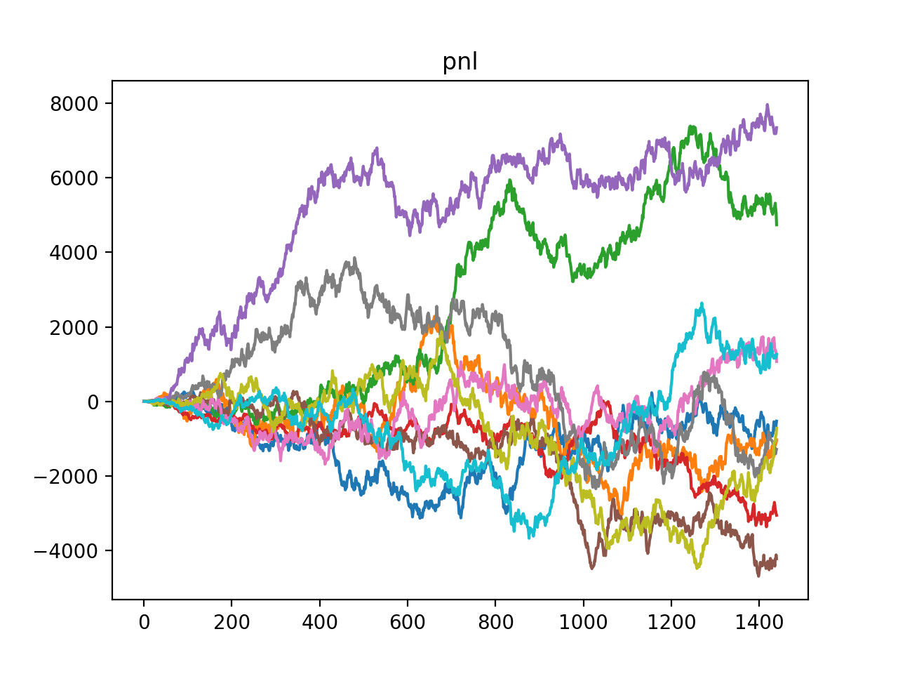
    plt.figure()
    plt.plot(Display_pnl)
    plt.title('pnl')

    plt.show()