Optimal Execution with Nonlinear Impact

How to trade under nonlinear temporary impact and terminal penalization

In a previous post we examined how to optimally execute a buy order of Q share, with a limit price, a nonlinear temporary market impact function, and no time constraint (I wrote about the time-constrained case with linear market impact in this post) . This week, we look at the case where we do have a time constraint, and a penalty at expiry (we need to send a market order for any remaining shares to buy). We will examine the theoretical solution in the general case (nonlinear impact), and provide a closed-form solution if the market impact is linear.

Our setup is the same as in the previous post, namely, we want to buy Q shares of a stock S with mid price s_t, before time t=T. For convenience, we denote by q_t the negative inventory q_t = Q minus our current inventory (so that we start at q_0 = Q and end up at 0), and by x_t our cash account. These stochastic processes satisfy

\((1)\ \ \ \ \ \ \ \begin{equation*} \left\{ \begin{split} &ds_t = \sigma dW_t\\ \\ &dq_t = -\lambda_t dt;\ q_0=Q;\ dq_t\le 0;\ \lambda_t\ge 0\\ \\ &dx_t = -(s_t + f(\lambda_t))\lambda_t dt, \end{split} \right. \end{equation*}\)

where σ is the stock volatility and f(λ_t) is the temporary market impact function, as a function of the speed of buying λ_t. We are seeking to maximize our pnl

\((2)\ \ \ \ \ \ u(s,x,q,t) = \sup_{\{\lambda_t\}}\mathbb{E}_{s,x,q,t}\left(x_T - s_T q_T - \mu q_T^2\right),\)

where the penalization term μ>0 can be interpreted the following way: μ q_T is the spread we’ll pay to acquire any remaining inventory q_T at time T.

It is standard to show that u is the solution to the Hamilton-Jacobi-Bellman problem

\((3)\ \ \ \ \ \ \ \ \begin{equation*} \left\{ \begin{split} &u_t + \frac{\sigma^2}{2}u_{ss} + \sup_\lambda\left(-\lambda u_q - \left(s + f(\lambda)\right)\lambda u_x\right) = 0\\ \\ &u(s,x,q,t=T) = x - sq - \mu q^2. \end{split} \right. \end{equation*}\)

We now make the Ansatz

\((4)\ \ \ \ \ \ u(s,x,q,t) = x - sq - h(q,\tau),\ \ \ \tau = T - t,\)

and find that h(q,τ) satisfies

\((5)\ \ \ \ \ \ \begin{equation*} \left\{ \begin{split} &h_\tau + \sup_\lambda\left(\lambda h_q - F(\lambda)\right) = 0\\ \\ &h(q,0) = \mu q^2, \end{split} \right. \end{equation*}\)

where F(λ) = f(λ)λ. This can be rewritten

\((6)\ \ \ \ \ \ \begin{equation*} \left\{ \begin{split} &h_\tau + F^*(h_q) = 0\\ \\ &h(q,0) = \mu q^2, \end{split} \right. \end{equation*}\)

where F* is the Legendre-Fenchel transform of F:

\((7) \ \ \ \ \ \ \ F^*(p) = \sup_{q}\left(pq - F(q)\right).\)

Let’s assume now F is convex. This makes it quite convenient, since then F** = F, and the unique solution to (6) is given by the Hopf-Lax formula

\((8)\ \ \ \ \ \ h(q,\tau) = \inf_p\left(\tau F\left(\frac{p}{\tau}\right) + \mu (q-p)^2\right).\)

Once h(q,τ) is computed, the optimal speed of trading λ* = λ*(q,τ) can be inferred from (5):

\((9)\ \ \ \ \ \ F’(\lambda^*) = h_q.\)

Let’s explore closed-form solutions to (8) and (9) in the linear market impact case, namely f(λ) = θλ, F(λ) = θλ^2. In this case

\((10)\ \ \ \ \ \ \begin{equation*} \begin{split} h(q,\tau) &= \inf_p\left( \theta \tau^{-1} p^2 + \mu (q-p)^2\right)\\ \\ &=\frac{\theta}{\frac{\theta}{\mu} + \tau} q^2, \end{split} \end{equation*} \)

so that the optimal trading speed λ* is found to be (using (9)):

\(\boxed{(11)\ \ \ \ \ \ \lambda^* = \frac{1}{\frac{\theta}{\mu} + \tau} q.}\)

Close to maturity (τ=0), λ* is simply the remaining inventory times the ratio between the terminal penalty μ and the linear market impact constant θ, which means the larger the penalty, the faster we’ll trade. And, when we have time on our hands we can afford to trade more slowly and thereby reduce market impact, which is also reflected in (11). Let’s plot now this optimal speed (T = 1)

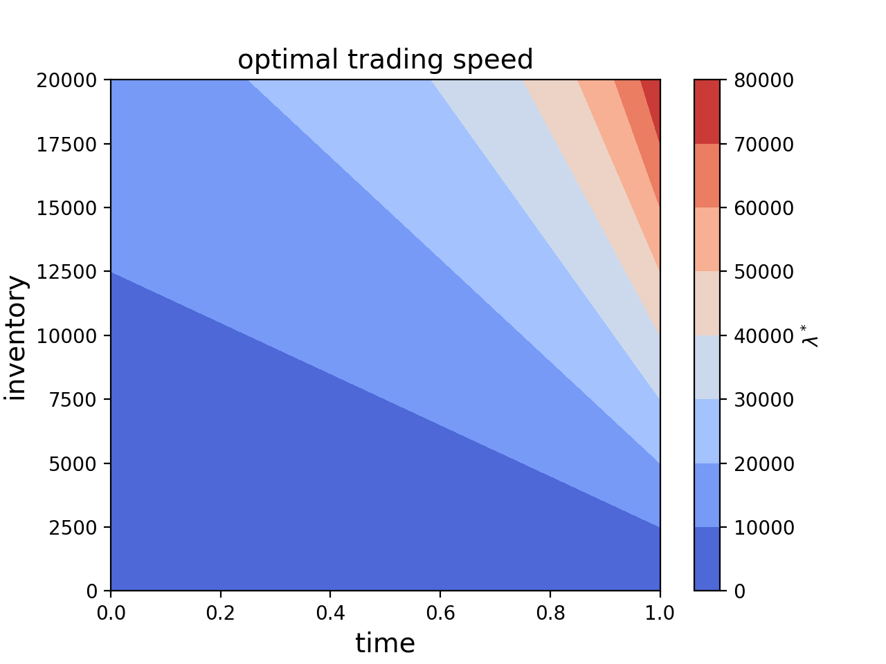
(Python code below the fold for paying subscribers.)

Quantitatively Yours,

---

from __future__ import print_function
import numpy as np
import matplotlib.pyplot as plt

DisplayPlots = True
q_min = 0
q_max = 20000
nq = 100
t_min = 0
t_max = 1 
nt = 150
theta_over_mu = 0.25
lam = np.zeros((nt,nq))
q_pts = np.linspace(q_min,q_max,nq)
t_pts = np.linspace(t_min,t_max,nt)
for i in range(nt):
    t = t_pts[i]
    for j in range(nq):
        q = q_pts[j]
        lam[i,j] = (1/(theta_over_mu + (t_max - t))) * q


if DisplayPlots:

    q, t = np.meshgrid(q_pts, t_pts)   
    # Plot the contour
    plt.figure()
    contour_plot = plt.contourf(t, q,lam, cmap='coolwarm')
    plt.colorbar(contour_plot, label=r'$\lambda^*$')
    plt.title('optimal trading speed', fontsize=14)
    plt.xlabel('time', fontsize=14)
    plt.ylabel('inventory', fontsize=14)
    plt.show()